Published on 9 September 2026

The various height systems – an overview and some theoretical concepts

In geodesy, the vertical distance between a point and a reference surface is called altitude or height. There are different height systems depending on the chosen reference surface and the consideration of gravitational potential in the calculation. Here is a brief overview, partly mathematical.

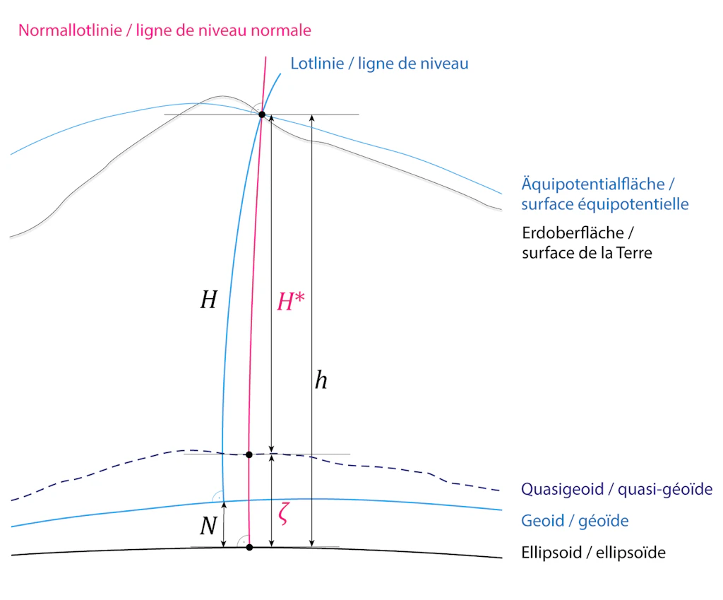
In geodesy, two main categories of altitudes are distinguished: geometric altitudes and physical altitudes.

Geometric Altitudes

Geometric altitudes, expressed as ellipsoidal heights, are directly measurable by global satellite positioning methods such as GNSS. Their main disadvantage is that they do not allow easy access to gravitational potential energy levels (equipotential surfaces), which are essential in practical applications. For example, water can flow between two points located at the same ellipsoidal height.

Physical Altitudes

Physical altitudes take into account Earth's gravity and aim to define the altitude of points so that water cannot flow between two points at the same altitude. Depending on the type of measurement (levelling, GPS) and the reference surface, physical altitude is distinguished into:

• Usual altitudes

• Dynamic altitudes

• Orthometric altitudes

• Normal altitudes

These different systems each have theoretical and practical advantages and disadvantages, but share the common basis of being founded on the geopotential number.

The Geopotential Number

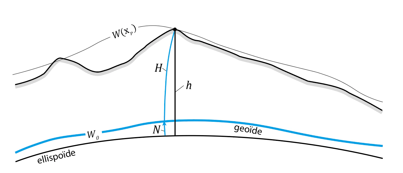
The geopotential number C of a point P at position x_P is defined as the difference between the gravity potential at the reference level (the geoid), denoted W₀, and the potential W at point P.

C(x_P) = W₀ – W(x_P)

It is expressed inm²/s². ². A geopotential number can be obtained, for example, by geometric levelling measurements combined with gravimetric data, by multiplying the height differences (expressed in metres) by local values of the acceleration of gravity (in m/s²).

To obtain an altitude H, one simply divides the geopotential number by the reference gravity acceleration G_0.

H(x_P) = C(x_P) / G₀

Depending on how G₀ is calculated, different types of altitudes are obtained, as presented below.

Usual Altitudes

A simple method to obtain physical altitudes is to perform geometric levelling measurements. A major problem with so-called “usual” altitudes is that they are not unique: the altitude of a point depends on the path taken to level it. Consequently, the altitude cannot be derived from the geopotential number either. In other words, even without any measurement uncertainty, the same point can be assigned different altitudes depending on the path followed.

The first precision levelling of Switzerland was carried out between 1860 and 1890. The altimetric system currently in force in Switzerland, LN02 (national levelling of 1902), is based on usual altitudes. The erratic block “Pierre du Niton”, located in the Geneva lake basin, serves as the reference point for altitude determination.

Dynamic Altitudes

If a constant γ₀ (generally 9,806 m/s²) is chosen for G₀, the following dynamic altitudes are obtained:

H^dyn(x_P) = C(x_P) / γ₀

Only dynamic altitudes allow rigorous access to the gravitational potential energy level. Because of this property, one might think that dynamic altitudes constitute the ideal altitudes. Unfortunately, in practice, they are not ideal. Indeed, the differences between dynamic altitude and vertical distances measured by geometric levelling are significant even for small paths. One would therefore have to systematically go through the geopotential number to obtain the dynamic altitude. It is for this practical reason that orthometric and normal altitudes are used instead. They make a slight compromise on the equality between equipotential surfaces and equal-altitude surfaces in favour of a good correspondence between geometric vertical distances and altitude differences.

Orthometric Altitudes

If the mean acceleration of gravity along the plumb line g̅ is used for G₀, the following orthometric altitudes are obtained:

H(x_P) = C(x_P) / g̅

However, this mean gravity acceleration cannot be determined directly by measurement, since it is impossible to access the Earth's interior. It is therefore necessary to resort to mass models integrating hypotheses on the density of rocks between the topography and the geoid, based on gravimetric measurements made at the surface.

Orthometric altitudes are unique and refer to the geoid, which is an equipotential surface corresponding to the ocean surface extended under the continents. Geometrically, the orthometric altitude H corresponds to the curvilinear distance along the plumb line between the considered point and its corresponding point on the geoid surface. It is related to the ellipsoidal height h by the geoid undulation N:

H = h – N

Normal Altitudes

If the mean normal acceleration along the plumb line g̅_n is used for G_0, the following normal altitudes are obtained:

H*(x_P) = C(x_P) / g̅_n

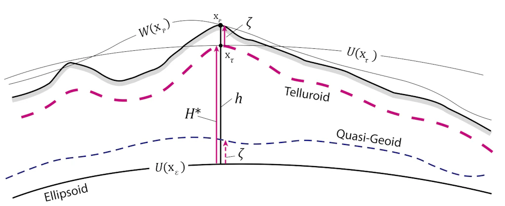
The main difficulty in determining orthometric altitudes lies in the precise estimation of the mean gravity g̅. To circumvent this limitation, the geodesist Mikhail Molodensky proposed in the 1960s an alternative system of unique physical altitudes, also based on geopotential numbers. This system replaces g̅ with the mean normal gravity acceleration g̅_n, calculated from a theoretical gravity field generated by a homogeneous ellipsoid of revolution whose mass is equivalent to that of the Earth. (See Normal altitudes for the Swiss height system)(see Des altitudes normales pour le système altimétrique suisse)

The advantage is that the mean normal gravity acceleration g̅_n can be obtained without uncertainty or hypotheses on the mass distribution in the Earth's crust.

Unlike orthometric altitudes, normal altitudes do not refer to the geoid, nor to any other equipotential surface. Their reference surface is called the quasi-geoid. Finally, to obtain a normal altitude from an ellipsoidal height h measured by GNSS, one applies a relation analogous to that used for orthometric altitudes. However, instead of the geoid undulation N, one subtracts the height anomaly 𝜁 :

H* = h – 𝜁